RNN Training, Advantages & Disadvantages (Complete Guidance)
Recurrent Neural Networks (RNN) are a part of a larger institution of algorithms referred to as sequence models. Sequence models made giant leaps forward within the fields of speech recognition, tune technology, DNA series evaluation, gadget translation, and plenty of extras.
What Are Recurrent Neural Networks (RNN)?
- RNN recalls the past and its selections are motivated with the aid of what it has learned from the past.
- Simple feed ahead networks “don’t forget” things too, however they consider things they learned at some stage in training.
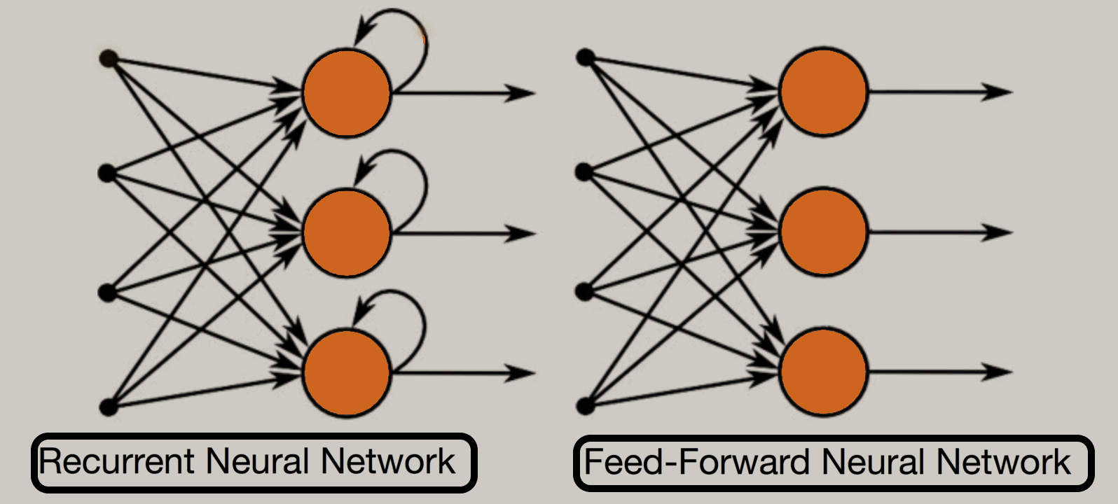
- A recurrent neural network appears very just like feedforward neural networks, except it also has connections pointing backwards.
- At each time step t (additionally called a frame), the RNN’s gets the inputs x(t) in addition to its personal output from the preceding time step, y(t–1). In view that there is no previous output at the primary time step, it’s far usually set to 0.
- Without difficulty, you can create a layer of recurrent neurons. At whenever step t, every neuron gets the entering vector x(t) and the output vector from the previous time step y(t–1).
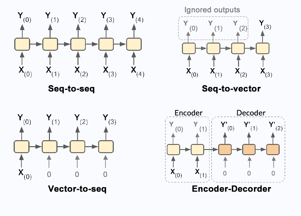
Input And Output Sequences of RNN
- An RNN can concurrently take a series of inputs and produce a series of outputs.
- This form of sequence-to-sequence network is useful for predicting time collection which includes stock prices: you feed it the costs during the last N days, and it ought to output the fees shifted by means of sooner or later into the future.
- You may feed the network a series of inputs and forget about all outputs besides for the final one, words, that is a sequence-to-vector network.
- You could feed the network the equal input vector again and again once more at whenever step and allow it to output a sequence, that is a vector-to-sequence network.
- You can have a sequence-to-vector network, referred to as an encoder, followed by a vector-to-sequence network, called a decoder.
Also Read : Azure DevOps Vs AWS DevOps
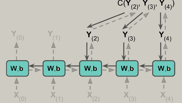
Training Recurrent Neural Networks (RNN)
- To train an RNN, the trick is to unroll it through time and then actually use regular backpropagation. This strategy is known as backpropagation through time (BPTT).
- There’s a first forward pass via the unrolled network. Then the output sequence is evaluated with the use of a cost function C.
- The gradients of that cost feature are then propagated backwards via the unrolled network.
- Now the model parameters have updated the use of the gradients computed all through BPTT.
Why Recurrent Neural Networks?
Recurrent Neural Networks have unique capacities as opposed to other kinds of Neural Networks, which open a wide range of possibilities for their users still also bringing some challenges with them. Then’s a rundown of the main benefits
- It’s the only neural network with memory and binary data processing.
- It can plan out several inputs and productions. Unlike other algorithms that deliver one product for one input, the benefit of RNN is that it can plot out many to many, one to many, and many to one input and productions.
How Does Recurrent Neural Networks Work
In Recurrent Neural networks, the data cycles through a loop to the center hidden layer.
The input layer ‘x’ takes within the input to the neural network and processes it and passes it onto the center layer.
The middle layer ‘h’ can encompass multiple hidden layers, each with its own activation functions and weights and biases. If you have got a neural network where the assorted parameters of various hidden layers aren’t tormented by the previous layer, ie: the neural network doesn’t have memory, then you’ll be able to use a recurrent neural network.
The Recurrent Neural Network will standardize the various activation functions and weights and biases in order that each hidden layer has the identical parameters. Then, rather than creating multiple hidden layers, it’ll create one and loop over it as over and over as needed.
Feed-Forward Neural Networks vs Recurrent Neural Networks
A feed-forward neural network allows information to flow only within the forward direction, from the input nodes, through the hidden layers, and to the output nodes. There aren’t any cycles or loops within the network.
Below is how a simplified presentation of a feed-forward neural network looks like:
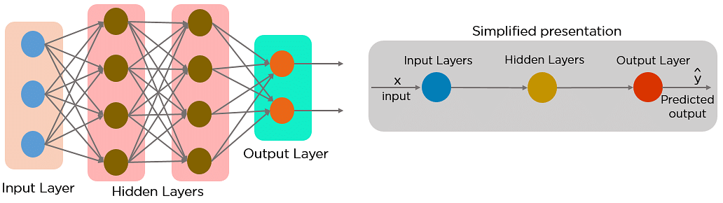
In a feed-forward neural network, the choices are supported this input. It doesn’t memorize the past data, and there’s no future scope. Feed-forward neural networks are utilized in general regression and classification problems.
Types of Recurrent Neural Networks
There are four types of Recurrent Neural Networks:
- One to One
- One to Many
- Many to One
- Many to Many
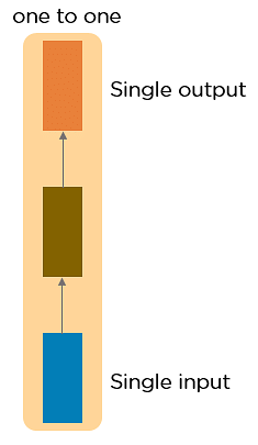
One to One RNN
This type of neural network is understood because the Vanilla Neural Network. It’s used for general machine learning problems, which contains a single input and one output.
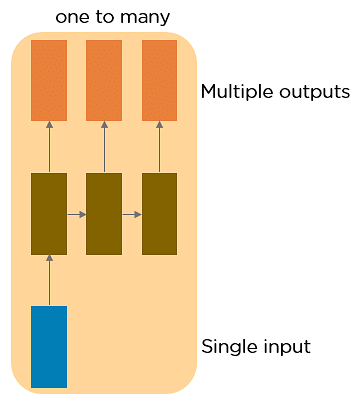
One to Many RNN
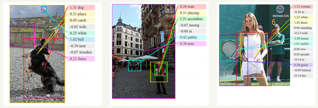
This type of neural network incorporates a single input and multiple outputs. An example of this is often the image caption.
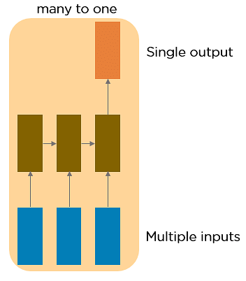
Many to One RNN
This RNN takes a sequence of inputs and generates one output. Sentiment analysis may be a example of this sort of network where a given sentence are often classified as expressing positive or negative sentiments.
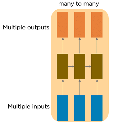
Many to Many RNN
This RNN takes a sequence of inputs and generates a sequence of outputs. artificial intelligence is one among the examples.
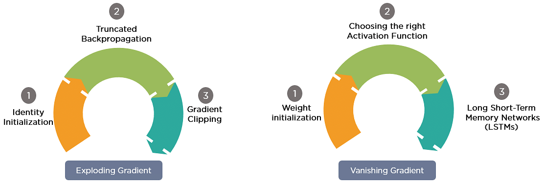
Two Issues of Standard RNNs
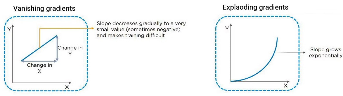
1. Vanishing Gradient Problem
Recurrent Neural Networks enable you to model time-dependent and sequential data problems, like stock exchange prediction, artificial intelligence, and text generation. you’ll find, however, RNN is tough to train due to the gradient problem.
RNNs suffer from the matter of vanishing gradients. The gradients carry information utilized in the RNN, and when the gradient becomes too small, the parameter updates become insignificant. This makes the training of long data sequences difficult.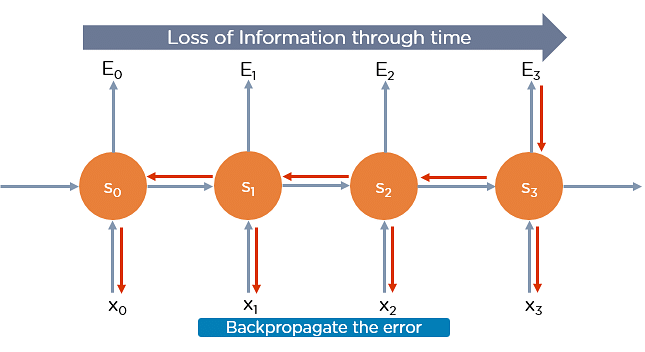
2. Exploding Gradient Problem
While training a neural network, if the slope tends to grow exponentially rather than decaying, this is often called an Exploding Gradient. This problem arises when large error gradients accumulate, leading to very large updates to the neural network model weights during the training process.
Long training time, poor performance, and bad accuracy are the key issues in gradient problems.
Gradient Problem Solutions
Now, let’s discuss the foremost popular and efficient thanks to cope with gradient problems, i.e., Long immediate memory Network (LSTMs).
First, let’s understand Long-Term Dependencies.
Suppose you wish to predict the last word within the text: “The clouds are within the ______.”
The most obvious answer to the present is that the “sky.” We don’t need from now on context to predict the last word within the above sentence.
Consider this sentence: “I are staying in Spain for the last 10 years…I can speak fluent ______.”
The word you are expecting will rely on the previous couple of words in context. Here, you would like the context of Spain to predict the last word within the text, and also the most fitted answer to the present sentence is “Spanish.” The gap between the relevant information and also the point where it’s needed may became very large. LSTMs facilitate your solve this problem.
Backpropagation Through Time
Backpropagation through time is once we apply a Backpropagation algorithm to a Recurrent Neural network that has statistic data as its input.
In a typical RNN, one input is fed into the network at a time, and one output is obtained. But in backpropagation, you utilize this additionally because the previous inputs as input. this is often called a timestep and one timestep will contains many statistic data points entering the RNN simultaneously.
Once the neural network has trained on a timeset and given you an output, that output is employed to calculate and accumulate the errors. After this, the network is rolled duplicate and weights are recalculated and updated keeping the errors in mind.
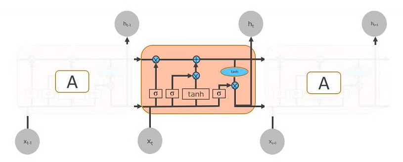
Long Short-Term Memory (LSTM)
- A unique kind of Recurrent Neural Networks, capable of learning lengthy-time period dependencies.
- LSTM’s have a Nature of Remembering facts for a long interval of time is their Default behaviour.
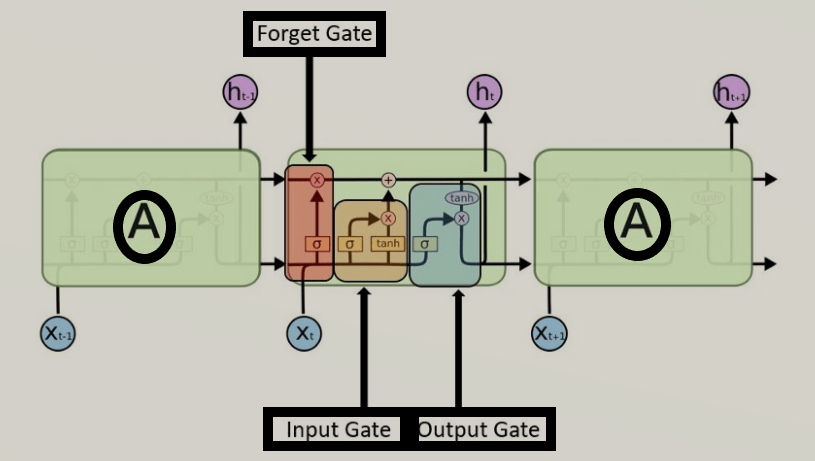
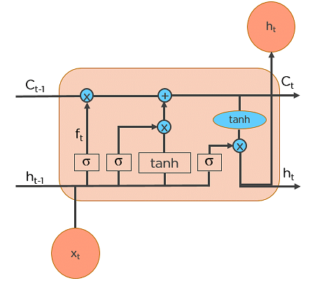
- Each LSTM module may have three gates named as forget gate, input gate, output gate.
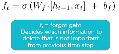
- Forget Gate: This gate makes a decision which facts to be disregarded from the cellular in that unique timestamp. it’s far determined via the sigmoid function.
- Input gate: makes a decision how plenty of this unit is introduced to the current state. The sigmoid function makes a decision which values to permit through 0,1. and Tanh function gives weightage to the values which might be handed figuring out their level of importance ranging from-1 to at least one.
- Output Gate: comes to a decision which a part of the current cell makes it to the output. Sigmoid characteristic decides which values to permit thru zero,1. and Tanh characteristic gives weightage to the values which can be exceeded determining their degree of importance ranging from-1 to at least one and expanded with an output of Sigmoid.
Workings of LSTMs in RNN
Step 1: Decide How Much Past Data It Should Remember
The first step within the LSTM is to determine which information should be omitted from the cell therein particular time step. The sigmoid function determines this. it’s at the previous state (ht-1) together with the present input xt and computes the function.
Consider the subsequent two sentences:
Let the output of h(t-1) be “Alice is good in Physics. John, on the opposite hand, is nice at Chemistry.”
Let the present input at x(t) be “John plays football well. He told me yesterday over the phone that he had served because the captain of his college team.”
The forget gate realizes there may well be a change in context after encountering the primary punctuation mark. It compares with the present input sentence at x(t). the subsequent sentence talks about John, that the information on Alice is deleted. The position of the topic is vacated and assigned to John.
Step 2: Decide How Much This Unit Adds to the Current State
In the second layer, there are two parts. One is that the sigmoid function, and also the other is that the tanh function. within the sigmoid function, it decides which values to let through (0 or 1). tanh function gives weightage to the values which are passed, deciding their level of importance (-1 to 1).
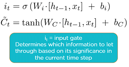
With the present input at x(t), the input gate analyzes the important information — John plays football, and also the incontrovertible fact that he was the captain of his college team is vital.
“He told me yesterday over the phone” is a smaller amount importance; hence it’s forgotten. This process of adding some new information may be done via the input gate.
Step 3: Decide What Part of the Current Cell State Makes It to the Output
The third step is to determine what the output are. First, we run a sigmoid layer, which decides what parts of the cell state make it to the output. Then, we put the cell state through tanh to push the values to be between -1 and 1 and multiply it by the output of the sigmoid gate.

Let’s consider this instance to predict the subsequent word within the sentence: “John played tremendously well against the opponent and won for his team. For his contributions, brave ____ was awarded player of the match.”
There can be many choices for the empty space. this input brave is an adjective, and adjectives describe a noun. So, “John” can be the most effective output after brave.
LSTM Use Case
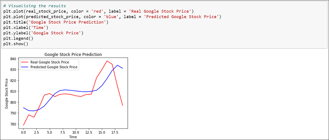
Now that you just understand how LSTMs work, let’s do a practical implementation to predict the costs of stocks using the “Google stock price” data.
Based on the stock price data between 2012 and 2016, we are going to predict the stock prices of 2017.
1. Import the desired libraries

2. Import the training dataset

3. Perform feature scaling to remodel the information

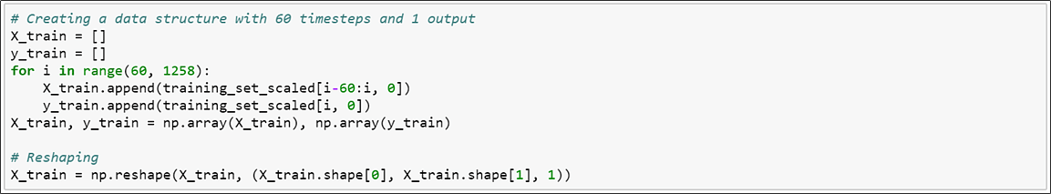
4. Create an information structure with 60-time steps and 1 output
5. Import Keras library and its packages
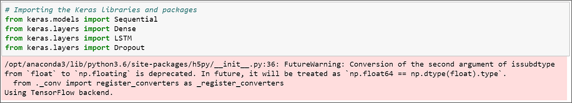
6. Initialize the RNN

7. Add the LSTM layers and a few dropout regularization.
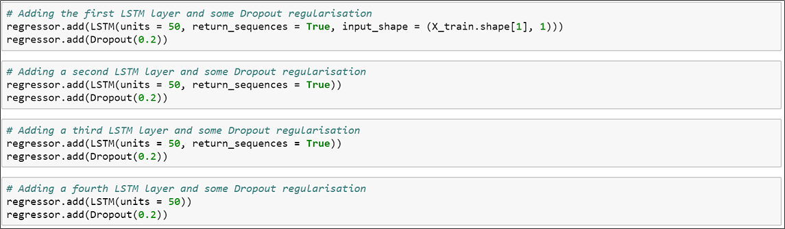
8. Add the output layer.

9. Compile the RNN

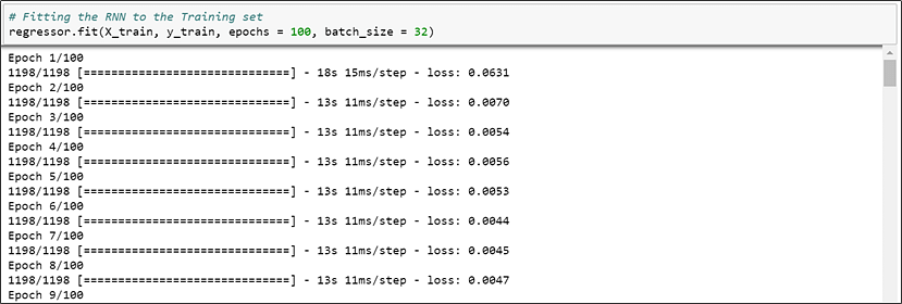
10. Fit the RNN to the training set
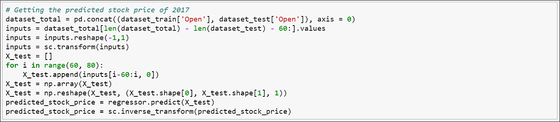
11. Load the stock price test data for 2017

12. Get the anticipated stock price for 2017
13. Visualize the results of predicted and real stock price
Advantages Of RNN’s
- The principal advantage of RNN over ANN is that RNN can model a collection of records (i.e. time collection) so that each pattern can be assumed to be dependent on previous ones.
- Recurrent neural networks are even used with convolutional layers to extend the powerful pixel neighbourhood.
Disadvantages of RNN’s
- Gradient exploding and vanishing problems.
- Training an RNN is a completely tough task.
- It cannot system very lengthy sequences if the usage of Tanh or Relu as an activation feature.
Applications 0f RNN’s
- Text Generation
- Machine Translation
- Visual Search, Face detection, OCR
- Speech recognition
- Semantic Search
- Sentiment Analysis
- Anomaly Detection
- Stock Price Forecasting
Frequently Asked Questions (FAQs)
Q1. What’s the Difference Between a Feedforward Neural Network and Recurrent Neural Network?
In this deep learning interview question, the interviewee expects you to relinquish an in depth answer.
- A Feedforward Neural Network signals travel in one direction from input to output. There are not any feedback loops; the network considers only this input. It cannot memorize previous inputs (e.g., CNN).
- A Recurrent Neural Network’s signals travel in both directions, creating a looped network. It considers this input with the previously received inputs for generating the output of a layer and might memorize past data because of its internal memory.
Q2. What Are the Applications of a Recurrent Neural Network (RNN)?
The RNN are often used for sentiment analysis, text mining, and image captioning. Recurrent Neural Networks also can address statistic problems like predicting the costs of stocks during a month or quarter.
Q3. What Are the Softmax and ReLU Functions?
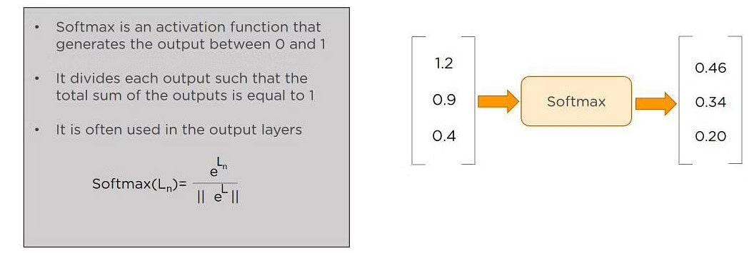
Softmax is an activation function that generates the output between zero and one. It divides each output, specified the whole sum of the outputs is adequate to one. Softmax is usually used for output layers.
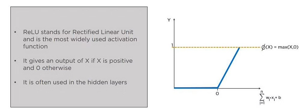
 ReLU (or Rectified Linear Unit) is that the most generally used activation function. It gives an output of X if X is positive and zeros otherwise. ReLU is commonly used for hidden layers.
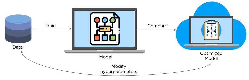
 Q4. What Are Hyperparameters?
This is another commonly asked deep learning interview question. With neural networks, you’re usually working with hyperparameters once the information is formatted correctly. A hyperparameter may be a parameter whose value is about before the educational process begins. It determines how a network is trained and also the structure of the network (such because the number of hidden units, the training rate, epochs, etc.).
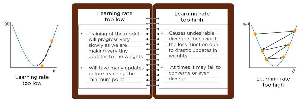
 Q5. What’s going to Happen If the training Rate is ready Too Low or Too High?
When your learning rate is simply too low, training of the model will progress very slowly as we are making minimal updates to the weights. it’ll take many updates before reaching the minimum point.
If the training rate is ready too high, this causes undesirable divergent behavior to the loss function thanks to drastic updates in weights. it’s going to fail to converge (model can provides a good output) or perhaps diverge (data is simply too chaotic for the network to train).
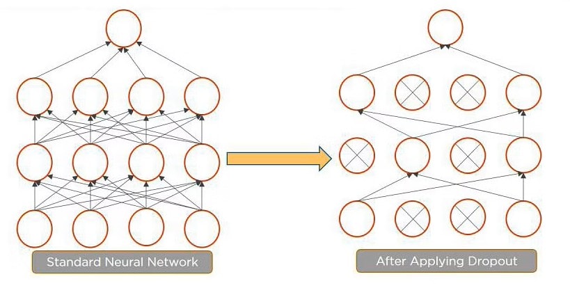
 Q6. What’s Dropout and Batch Normalization?
Dropout could be a technique of dropping by the wayside hidden and visual units of a network randomly to stop overfitting of information (typically dropping 20 percent of the nodes). It doubles the quantity of iterations needed to converge the network.
 Batch normalization is that the technique to enhance the performance and stability of neural networks by normalizing the inputs in every layer in order that they need mean output activation of zero and variance of 1.
Q7. What’s Overfitting and Underfitting, and the way to Combat Them?
Overfitting occurs when the model learns the main points and noise within the training data to the degree that it adversely impacts the execution of the model on new information. it’s more likely to occur with nonlinear models that have more flexibility when learning a target function. An example would be if a model is watching cars and trucks, but only recognizes trucks that have a selected box shape. it would not be ready to notice a flatbed truck because there’s only a selected quite truck it saw in training. The model performs well on training data, but not within the universe.
Underfitting alludes to a model that’s neither well-trained on data nor can generalize to new information. This usually happens when there’s less and incorrect data to coach a model. Underfitting has both poor performance and accuracy.
To combat overfitting and underfitting, you’ll resample the info to estimate the model accuracy (k-fold cross-validation) and by having a validation dataset to judge the model.
Q8. How Are Weights Initialized in an exceedingly Network?
There are two methods here: we are able to either initialize the weights to zero or assign them randomly.
- Initializing all weights to 0: This makes your model almost like a linear model. All the neurons and each layer perform the identical operation, giving the identical output and making the deep net useless.
- Initializing all weights randomly: Here, the weights are assigned randomly by initializing them very near 0. It gives better accuracy to the model since every neuron performs different computations. this is often the foremost commonly used method.
Q9. What Are the various Layers on CNN?
There are four layers in CNN:
- Convolutional Layer – the layer that performs a convolutional operation, creating several smaller picture windows to travel over the info.
- ReLU Layer – it brings non-linearity to the network and converts all the negative pixels to zero. The output could be a rectified feature map.
- Pooling Layer – pooling may be a down-sampling operation that reduces the dimensionality of the feature map.
- Fully Connected Layer – this layer recognizes and classifies the objects within the image.
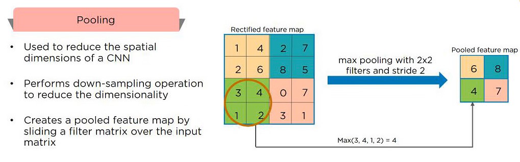
Q10. what’s Pooling on CNN, and the way Does It Work?
Pooling is employed to scale back the spatial dimensions of a CNN. It performs down-sampling operations to cut back the dimensionality and creates a pooled feature map by sliding a filter matrix over the input matrix.
 Q11. How Does an LSTM Network Work?
Long-Short-Term Memory (LSTM) could be a special reasonably recurrent neural network capable of learning long-term dependencies, remembering information for long periods as its default behavior. There are three steps in an LSTM network:
- Step 1: The network decides what to forget and what to recollect.
- Step 2: It selectively updates cell state values.
- Step 3: The network decides what a part of this state makes it to the output.
 Q12. What Are Vanishing and Exploding Gradients?
While training an RNN, your slope can become either too small or too large; this makes the training difficult. When the slope is simply too small, the matter is thought as a “Vanishing Gradient.” When the slope tends to grow exponentially rather than decaying, it’s remarked as an “Exploding Gradient.” Gradient problems cause long training times, poor performance, and low accuracy.
 Q13. what’s the Difference Between Epoch, Batch, and Iteration in Deep Learning?
Epoch – Represents one iteration over the whole dataset (everything put into the training model).
Batch – Refers to once we cannot pass the whole dataset into the neural network directly, so we divide the dataset into several batches.
Iteration – if we’ve got 10,000 images as data and a batch size of 200. then an epoch should run 50 iterations (10,000 divided by 50).